Morpho: massive improvements in performance of semi-landmark sliding
31 Oct 2014On my visit of the MPI in Leipzig (which was great, thanks a lot!!), Philip Gunz told me about a method (proposed by Demetris Halazonetis) that could improve computation time and memory footprint for the relaxation of semi-landmarks, which are serious restrictions on the maximum amount of coordinates usable with this method. So I spent the best part of Wednesday night and the 6-hour train ride home to tweak the underlying subroutines, making use of the excellent R-package Matrix and its large variety of classes for all kinds of sparse/triangle/symmetric matrices.
At the end I was able to run the examples in my package on my netbook as fast as the untweaked version on my desktop workstation.
So when I arrived at the office this morning, I was eager to compare benchmarks between those version on my machine.
Hardware specs:
- CPU: Intel(R) Xeon(R) CPU E5-1650 v2 @ 3.50GHz (Hexacore)
- RAM: 32GB DDR3 @1600 MHz
Software:
- Ubuntu 14.04.1
- Vanilla R 3.1.1
- BLAS: ATLAS tuned to my machine (it is definitely worth it!!) to allow parallel algebra operations.
### first create a benchmarking function

benchslide <- function(nofl=c(50,100,200,500,1000,2000,3000,4000)) {
    require(Morpho)
    require(Rvcg)
    data(nose)
    tmp <- NULL
    for (i in 1 : length(nofl)) {
        cat(paste0("running function with ",nofl[i]," semi-landmarks\n"))
        semi <- vcgSample(shortnose.mesh,SampleNum = nofl[i])
        semilong <- tps3d(semi,shortnose.lm,longnose.lm)
        tmp[i] <- system.time(relax <- relaxLM(semi,semilong, mesh=shortnose.mesh, iterations=1,SMvector=1:nrow(semi), deselect=F,surp=1:nrow(semi)))[3]
        cat(paste0("finished with ",nofl[i]," in ", tmp[i], " seconds\n"))
    }
    return(list(timing=tmp,nofl=nofl))
}


### now install pretweaked version from github:
require(devtools)

install_github("zarquon42b/Morpho", ref="c8f3652bea901f40d93ce5efc645d2fb75b8a6da")

##run the benchmark function

old <- benchmark()
save(old,file="old")##save the results to disk


### now close the old workspace and open a new one

### get the tweaked version:
install_github("zarquon42b/Morpho", ref="ccb67d3f96d2810176490f32b0cdd0df66d51155")
new <- benchmark()
save(new,file="new")##save the results to disk

## now load timings from the old version and visualize them:
load("old")
plot(old$nofl,old$timing,col=2,cex=1.5,pch=19, xlab="no. of semi-landmarks", ylab="elapsed time in seconds")
lines(spline(old$nofl,old$timing),lwd=4,col=2)##create nice splines

load("new")#not necessary if you are still in your "new" workspace
points(new$nofl,new$timing,col=3,cex=1.5,pch=19)
lines(spline(new$nofl,new$timing),lwd=4,col=3)##create nice splines
Here are the graphs:
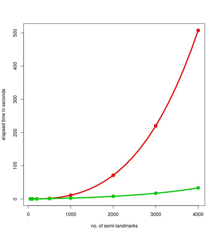
Hereby, the timing for 4000 semi-landmarks was 507.6 secs for the old version, compared to 33.5 secs for the tweaked version. Quite impressive, isn’t it?
FUN FACTS: using ATLAS and testing for 10,000 semi-landmarks with the tweaked function, I managed to max out all 32GB RAM (yay, first time on this machine). Using OpenBLAS, it only took 160 seconds (awesome!) and required only 20 GB RAM (don’t try this on your fancy tablets).
EXTRA FUN:
Now as a special gimmic, we calculate 2nd order polynomial approximations with number of landmarks as predictor in order to predict the timings for 10,000 semi-landmarks.
## first we check whether extrapolation of 2nd order Polynomial is sensible by calculating the model with the values for 4000 semi-landmarks removed and compare the resulting prediction with the actual value:
oldmod1 <- lm(old$timing[-8] ~ old$nofl[-8]+I(new$nofl[-8]^2))
newmod1 <- lm(new$timing[-8] ~ new$nofl[-8]+I(new$nofl[-8]^2))
pred4000old <- sum(oldmod1$coefficients*c(1,4000,4000^2))#426.4685 a bit underestimated compared to the actual value of 507.6
pred4000new <- sum(newmod1$coefficients*c(1,4000,4000^2))# 29.31068 reasonably close to the actual value of 33.5
### as the models tend to aim too low, the extrapolation will give us a lower boundary
### compute the models from the complete data
oldmod <- lm(old$timing ~ old$nofl+I(new$nofl^2))
newmod <- lm(new$timing ~ new$nofl+I(new$nofl^2))
## extrapolate from data
pred10000old <- sum(oldmod$coefficients*c(1,10000,10000^2))
pred10000new <- sum(newmod$coefficients*c(1,10000,10000^2))
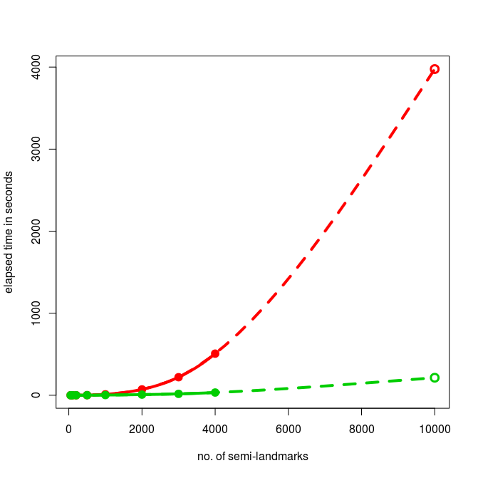
## create plot
oldnoflpred <- c(old$nofl,10000)
oldtimingpred <- c(old$timing,pred10000old)
newnoflpred <- c(new$nofl,10000)
newtimingpred <- c(new$timing,pred10000new)
plot(oldnoflpred,oldtimingpred,col=2,cex=0,pch=19, xlab="no. of semi-landmarks", ylab="elapsed time in seconds")
points(old$nofl,old$timing,col=2,cex=1.5,pch=19)
points(10000,pred10000old,col=2,cex=1.5,lwd=3)
lines(spline(old$nofl,old$timing),lwd=4,col=2)##create nice splines
lines(spline(oldnoflpred,oldtimingpred),lty=2,lwd=4,col=2)##create nice splines
points(new$nofl,new$timing,col=3,cex=1.5,pch=19)
points(10000,pred10000new,col=3,cex=1.5,lwd=3)
lines(spline(new$nofl,new$timing),lwd=4,col=3)##create nice splines
lines(spline(newnoflpred,newtimingpred),lty=2,lwd=4,col=3)##create nice splines
And here are the extrapolated timings for 10,000 landmarks: 213.7 secs with the tweaked function and 3975.83 secs for the old function (more than 1 hour).