Morpho: Determine meaningful Principal Components

As this is a somewhat longish post, here a table of content:

• Background
• Implementation
• Examples
• References

Background

Some time ago, I attended a talk of Fred Bookstein about separating meaningful PCs (eigenvectors of the covariance matrix) from those rather representing spherical noise. In this context “meaningful” means that the direction of the PC is distinctive. When reading biological/anthropological papers, one often finds detailed descriptions/analyses of shape changes associated with single PCs. This, however, presumes that these PCs have a mathematical meaning as distinctive axes of the ellipsoid representing the sample’s distribution. But what if the ellipsoid is rather a glorified sphere than a “real” ellipsoid? Then all analyses/interpretations based on single PCs are simply nonsensical.

This week, I got hold of a copy of Measuring and and reasoning by said Bookstein (2014), where the details (page 324f.) of the above mentioned talks are explained: The basic approach is based on a log-likelihood ratio. Without getting into the details, here is the shorthand version (also see Mardia et. al (1979; p. 235) for further theoretical details):

Be \(a\) the arithmetic mean of two eigenvalues and \(g\) their geometric mean and \(n\) the sample size, we then get a likelihood ratio \(2n*log \frac{a}{g} \) that can be approximated by a \( \chi^2 \)-Distribution of two degrees of freedom. To get a meaningful PC, only those eigenvectors are considered if the ratio between the corresponding eigenvalue and its successor (with the next lower eigenvalue) results in a log-likelihood ratio above the expected value of \(2\)- for a \( \chi^2 \)-Distribution with \(df=2\).

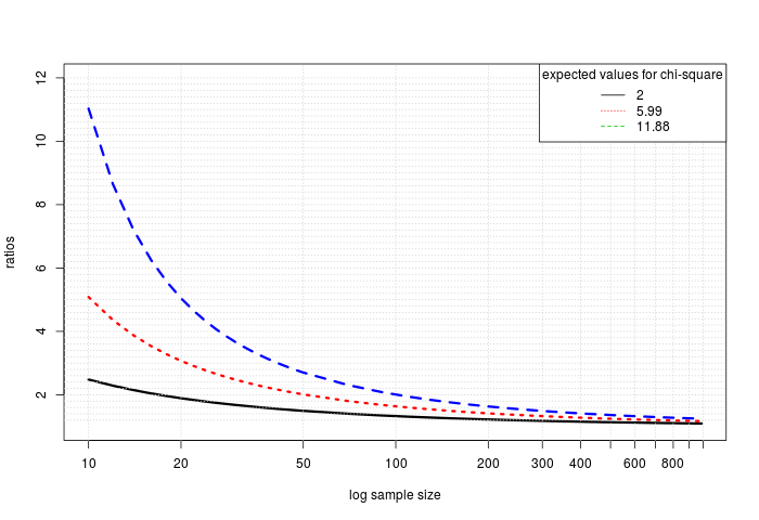
Enough theory, here are some examples, first we determine the ratios, depending on sample size, to attribute meaning to a PC, and then we compare it to the ratio necessary to consider the difference statistically significant.

Implementation

I implemented the method in the functions getMeaningfulPCs and getPCtol, with the latter calculating the ratio threshold given a specific sample size and expected value.

Examples

#get development snapshot of Morpho
require(devtools)
install_github("zarquon42b/Morpho")
require(Morpho)

## reproduce the graph from Bookstein (2014, p. 324)
## and then compare it to ratios for values to be considered
## statistically significant
     myseq <- seq(from=10,to = 50, by = 2)
     myseq <- c(myseq,seq(from=50,to=1000, by =20))
     ratios <- getPCtol(myseq)
     plot(log(myseq),ratios,cex=0,xaxt = "n",ylim=c(1,5.2))
     ticks <- c(10,20,50,100,200,300,400,500,600,700,800,900,1000)
     axis(1,at=log(ticks),labels=ticks)
     lines(log(myseq),ratios,lwd=3)
     abline(v=log(ticks), col="lightgray", lty="dotted")
     abline(h=seq(from=1.2,to=5, by = 0.2), col="lightgray", lty="dotted")
  
  
## now we raise the bar and compute the ratios for values
## to be beyond the 95th percentile of
## the corresponding chi-square distribution:
     ratiosSig <- getPCtol(myseq,expect=qchisq(0.95,df=2))
     lines(log(myseq),ratiosSig,col=2,lwd=3,lty=3)
     
    
##To be more anally retentive, we also correct for Type-I error inflation
## Let us assume we only check the first 20 PCs, we have 19 pairwise tests
## using the bonferroni-holm method, we have to lower the alpha value to 0.05/19=0.002631579
     padj <- 0.05/19
     ratiosSigAdj <- getPCtol(myseq,expect=qchisq(1-padj,df=2))
     lines(log(myseq),ratiosSigAdj,col=4,lwd=3,lty=2)

  ## add legend
     legend("topright",legend=as.character(round(c(2,qchisq(0.95,df=2),qchisq(1-padj,df=2)),digits=2)),title="expected values for chi-square",lty=c(1,3,2),col=1:3)

     

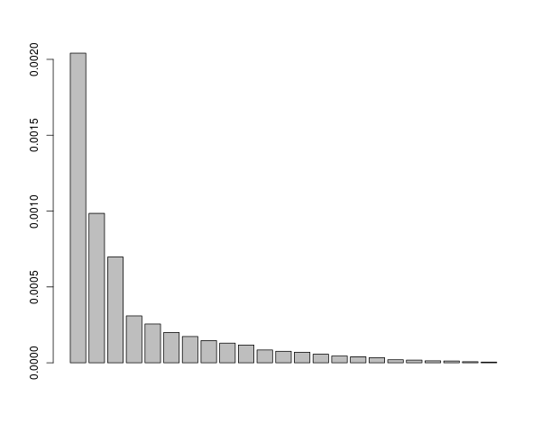
And finally a real world example: Get the number of meaningful PCs calculated from a set of superimposed landmarks.

require(Morpho)
data(boneData)

     proc <- procSym(boneLM)
     getMeaningfulPCs(proc$eigenvalues,n=nrow(proc$PCscores))
##output is
#    $tol #threshold for specific expected value and sample size 
#    [1] 1.372847
#    $good #indices of meaningful PCs
#    [1] 1 2 3
     ## the first 3 PCs are reported as meaningful
     ## show barplot that seem to fit the bill
     barplot(proc$eigenvalues)

References

[1] Bookstein, F. L. Measuring and reasoning: numerical inference in the sciences. Cambridge University Press, 2014

[2] Mardia, K. V.; Kent, J. T. & Bibby, J. M. Multivariate analysis. Academic press, 1979