mesheR and RvtkStatismo: added new shape model fitting algorithm

I implemented another function, called modelFitting (“where do they get these crazy names”), into mesheR to fit a statismo shape model to a target mesh. Other than the functions gaussMatch and AmbergRegister, here the model is not only used to regularize a free form deformation, but a (symmetric) mean squared distance between (iteratively updated closest points of) both meshes is minimized using an lbfgs optimizer.

Below are two examples (once again using Marcel’s femurs), one using landmarks to constrain a model and one where the target is initially registered to the model using a similarity and affine ICP.

###Example with a constrained model

require(RvtkStatismo)
require(mesheR)
require(Morpho)
ref <- read.vtk("VSD001_femur.vtk")
tar <- read.vtk("VSD002_femur.vtk")
ref.lm <- as.matrix(read.csv("VSD001-lm.csv",row.names=1))
tar.lm <- as.matrix(read.csv("VSD002-lm.csv",row.names=1))
mymod <- statismoModelFromRepresenter(ref,kernel=list(c(50,50)),ncomp = 100,isoScale = 0.1)
#constrain the model by the landmarks
mymodC <- statismoConstrainModel(mymod,tar.lm,ref.lm,2)
fit <- modelFitting(mymodC,tar,iterations = 15)
##create distance map
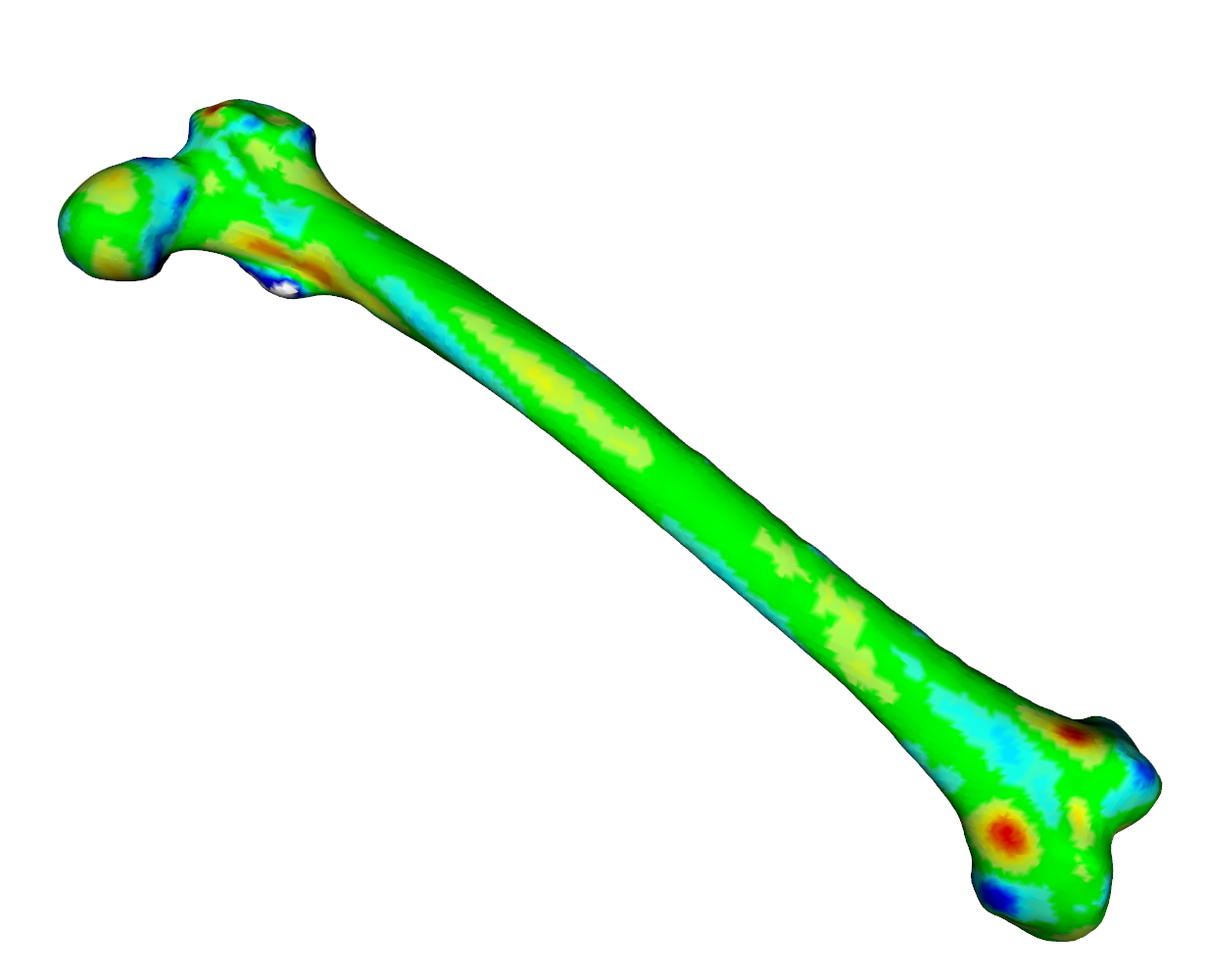
meshDist(fit$mesh,tar,from=-3,to=3,tol=0.5)

###Example initialized by a similarity and affine transform

#or without landmarks but instead with some icp steps
taricp <- icp(tar,ref,iterations = 50,type="s",getTransform = T)
taricpAff <- icp(taricp$mesh,ref,iterations = 50,type="a",getTransform = T)
##get affine transform
combotrafo <- taricpAff$transform%*%taricp$transform
fit2 <- modelFitting(mymod,taricpAff$mesh,iterations = 15)
## revert affine transforms
fit2aff <- applyTransform(fit2$mesh,combotrafo,inverse=T)
meshDist(fit2aff,tar,from=-3,to=3,tol=0.5)

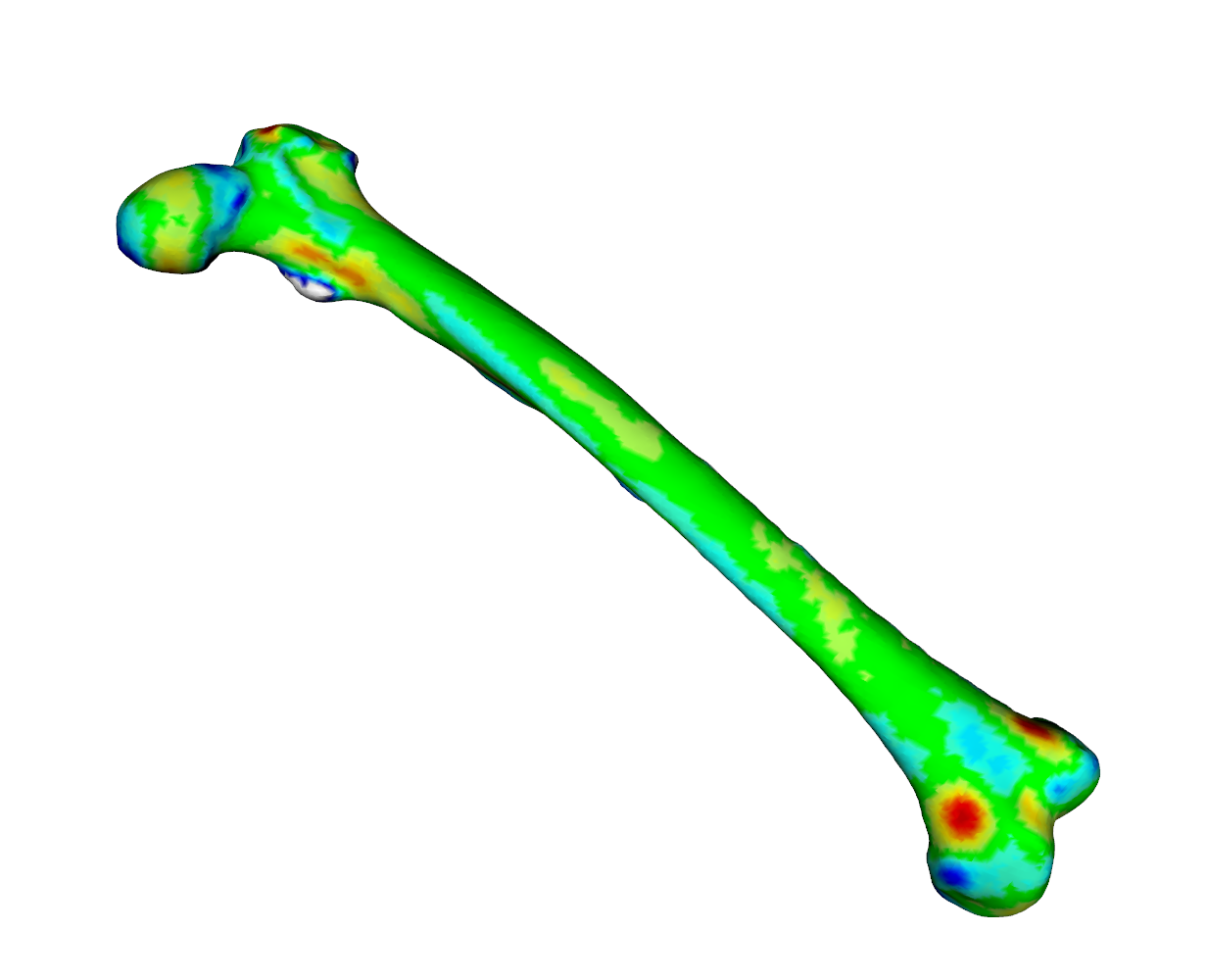
As we can see from the heatmaps in Fig. 1 an Fig. 2, the matched surfaces are very similar. But the visualization of the vertex differences between both matchings shows somewhat differing vertex positions (Fig 3):

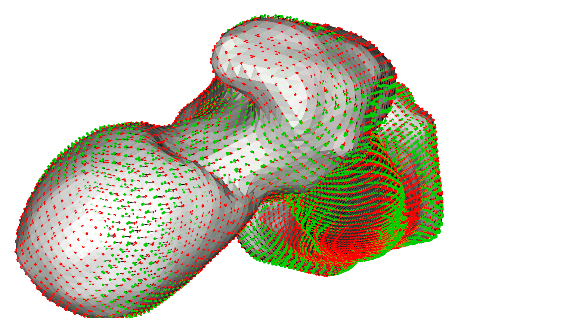
When I find some time, I will further add some regularizations regarding correspondence selection similar as in gaussMatch.