RvtkStatismo: Meet the new kernel interface

RvtkStatismo provides functions (statismoGPmodel and statismoModelFromRepresenter) that allow to extend/create a statistical model’s variability by combining sets of kernels (BSpline, Gaussian kernels, etc.). What was bugging me for a while was my clumsy implementation. I changed that and now the kernels (or rather the information how they are to be created/combined on C++ level) have their own interface in R. Instead of defining a list of parameters (which can get ugly), the workflow now is:

1. create your kernels
2. pass them to the respective function

In order to test this, you need

1. The development branch of statismo (ubuntu 14.04 users can install it from my ppa:

   sudo apt-add-repository ppa:zarquon42/statismo-develop	   
   sudo apt-get update   
   sudo apt-get install statismo
   

2. the development branch of RvtkStatismo In R issue:

   devtools::install_github("zarquon42b/Rvtkstatismo",ref="develop")
   

The following functions create matrix-valued kernels

• GaussianKernel
• BSplineKernel
• MultiscaleBSplineKernel
• IsoKernel
• StatisticalModelKernel

Those can be combined by:

• SumKernels
• ProductKernels

To allow expressions like \( (k_1 + k_2+ …+ k_n) * (k_{n+1}+…+k_m) * (…) \), with each \( k_i \) representing a matrix-valued kernel, one first creates the \( k_i \) and sums them up for each bracket. The summed up kernels can then be multiplied subsequently.

Example

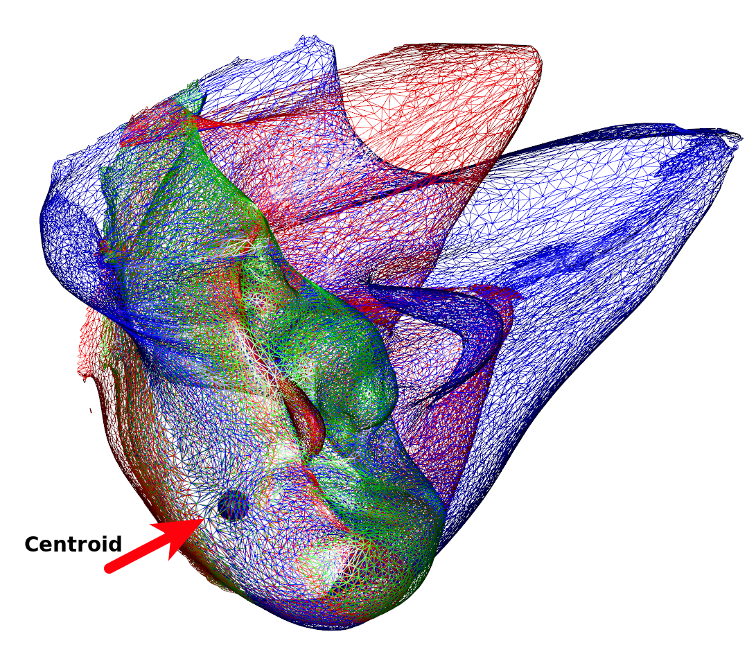
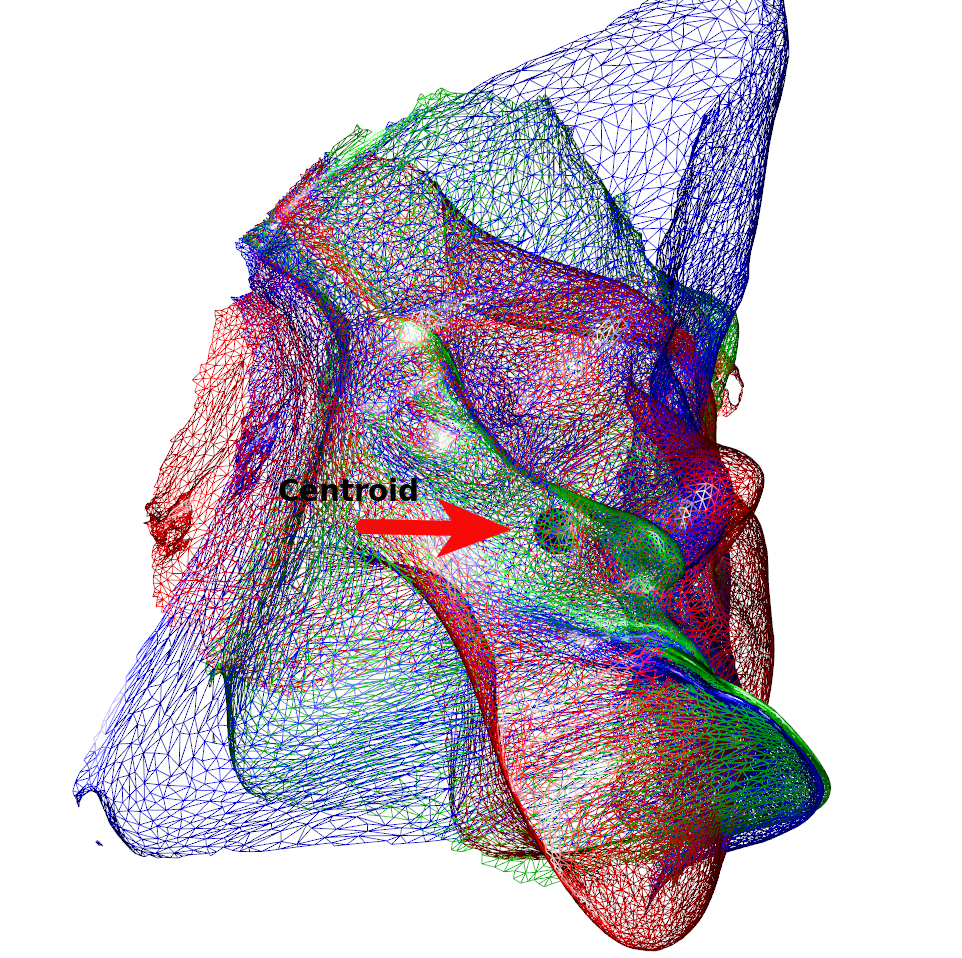
Below is a (rather nonsensical) example on how to combine different types of kernels (and create shapes resembling modern art). We can see that the variability is much less around the chin region (Figure 1). This is owed to the centroid of the isotropic kernel being close and with the displacement being a linear function of the distance to the center. By multiplying, we introduce dampening of the variability that increases the closer a point is to the centroid. If we use the original mesh’s center of gravity, we can see how this affects the resulting images (Figure 2).

require(RvtkStatismo)
require(Rvcg)
data(humface)
## create a Gaussian kernel and add it to a MultiscaleBSplineKernel kernel
k1 <- GaussianKernel(50,2)
k2 <- MultiscaleBSplineKernel(100,10,10)
sum1 <- SumKernels(k1,k2)

## create an Isotropic kernel and add it to a BSpline kernel
k3 <- IsoKernel(0.1,centroid=rep(0,3))
k4 <- BSplineKernel(100)
sum2 <- SumKernels(k3,k4)

productKernel <- ProductKernels(sum1,sum2)

## now create a Gaussian Process model from a mesh and sample some instances
gpmodel <- statismoModelFromRepresenter(humface,kernel=productKernel,ncomp=50)
for (i in 1:3) rgl::wire3d(DrawSample(gpmodel),col=i+1)

## show the centroid
spheres3d(rep(0,3),radius=5)

## now do the same but use an IsoKernel centered at the mesh's centroid
k3a <- IsoKernel(0.1,x=humface)
sum2a <- SumKernels(k3a,k4)

productKernel1 <- ProductKernels(sum1,sum2a)
gpmodela <- statismoModelFromRepresenter(humface,kernel=productKernel1,ncomp=50)
for (i in 1:3) rgl::wire3d(DrawSample(gpmodela),col=i+1)
## show the new centroid
spheres3d(k3a@centroid,radius=5)