More interpolations, fast subsampling and tweaking

General stuff

As can be seen in my last four posts, I started playing with displacement fields and interpolation. While the smoothers used so far provided fast and reasonable approximations, I wondered whether this could be improved/complemented by additional methods and starting digging into splines again. The nice thing about learning and the subsequent code revision is that you pick up quite some bug fixes and speed improvements along the way. For example: I realized that there was substantial tweaking potential in my Thin-Plate Spline function tps3d in Morpho, which now is much faster: Using 6000 control points, the deformation of a mesh with ~120000 vertices takes 16secs on my workstation (instead of ~90 secs before).

Fast K-means clustering for 2D and 3D data

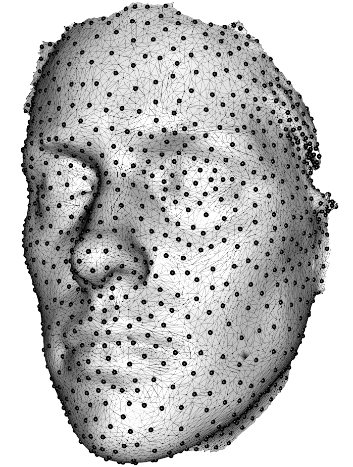
My idea was to subsample the displacement fields and calculate a TPS interpolation based on this subsampled data. Here, the next obstacle appeared: I could not find a fast way of getting nicely distributed sub-samples in R. R’s built in K-means clustering is too slow for large point clouds and large \(k\). So using the vcgKDtree function from Rvcg, I managed to implement a fast and parallel (thanks to OpenMP) K-means clustering algorithm that not only returns the K-means centers, but those points from the displacement field closest to these centers. Thus, the displacement field (or any point set) can be subsampled fast and leading to reasonable results (Figure 1 and Figure 2 show 1000 points sampled from a mesh).

require(Rvcg);require(Morpho)
data(humface)
clust <- fastKmeans(humface,k=1000,iter.max=100)
## plot the cluster centers
wire3d(humface)
spheres3d(clust$centers)
## now look at the vertices closest to the centers
spheres3d(vert2points(humface)[clust$selected,],col=2)
			 

Synthesis

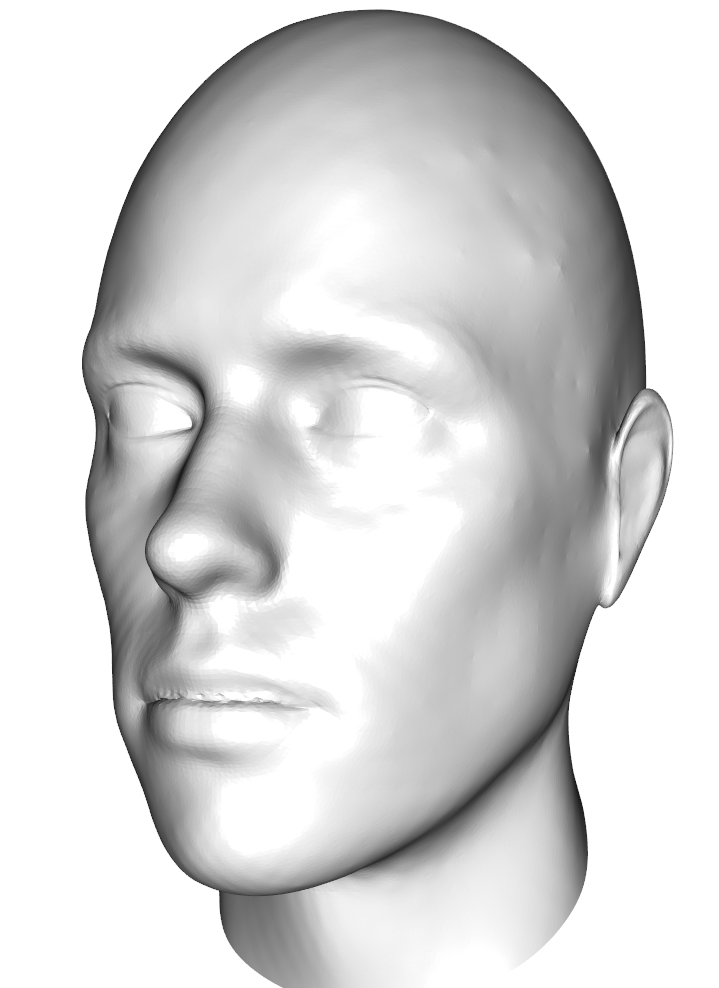
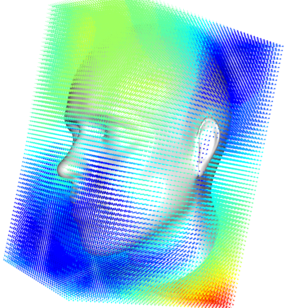
To throw all together, we can now do a fast subsampling of the displacement filed and compute a smooth TPS deformation (or smooth an existing one. In the next example, we will reuse the example from before, to interpolate a low resolution field. This time the resulting deformation leads instantaneously to a smooth surface (Figure 3). And additionally, we interpolate the highres field now to a cubic grid and add it to the plot (Figure 4).

highresdisp <- interpolateDisplacementField(dispfield,highres,type="TPS",subsample=4000)
highres_deformed <- applyDisplacementField(highresdisp,highres)
shade3d(highres_deformed,col="white")

## create a nice deformation grid
require(sp)
grid <- spsample(SpatialPoints(vert2points(highres)),100000,type="regular")
grid <- grid@coords
gridfield <- interpolateDisplacementField(highresdisp,grid,type = "TPS",subsample=4000)